Recent advances in generative foundational models, often termed “world models,” have propelled interest in applying them to critical tasks like robotic planning and autonomous system training. For reliable deployment, these models must exhibit high physical fidelity, accurately simulating real-world dynamics. Existing physics-based video benchmarks, however, suffer from entanglement, where a single test simultaneously evaluates multiple physical laws and concepts, fundamentally limiting their diagnostic capability. In addition, they typically rely on subjective VLM based judgements of the physical accuracy of the video.
We introduce WorldBench, a video-based benchmark specifically designed for concept-specific, disentangled evaluation, allowing us to isolate and assess understanding of a single physical concept or law at a time. To make WorldBench comprehensive, we design benchmarks at two levels:
Intuitive physics
How well do video generation models understand core physical principles?
425 simulated + 44 real
This subset targets four principles: motion physics, object permanence, support relations, and scale/perspective. It benchmarks a model’s ability to generate plausible dynamics governed by those core principles (e.g. a ball rolling behind pillars, an object moving toward the camera).
Metric: SAM2 masks vs. ground-truth segmentation (foreground mIoU) and background RMSE.
How well do video generation models represent exact physical constants?
234 real + 45 simulated
This subset requires the video to adhere to known physical parameters that govern the scene: gravitational acceleration, fluid viscosity, and friction coefficients. A physics simulator that generates incorrect gravity cannot be used to generate data for a model that needs to operate in the real world.
Metric: recover g, μ, and η from the generated video and compare them to known constants.
We introduce a video-based benchmark carefully designed to ensure each sample evaluates a single physics concept or constant, allowing for more fine-grained understanding of world-model physics.
We provide a dataset and codebase to estimate exact physical constants such as g from video, providing an absolute, meaningful metric to judge model performance as opposed to subjective (e.g. VLM judgment) or relative metrics.
We perform an empirical analysis of SOTA world foundation models and image-to-video models to identify concept-specific shortcomings and gaps in physical understanding, providing directions for future improvement.
Intuitive physics
The first subset assesses implicit understanding of core, foundational physics concepts, often referred to as “intuitive physics.” The goal is to determine if large-scale models, trained on vast quantities of video data, have internalized these cognitive building blocks. We focus on four concepts: motion physics (how objects move and interact), support relations (how objects are supported or balanced), object permanence (objects continue to exist when hidden), and scale/perspective (how size and spatial relationships change with motion or viewpoint).
For each concept we construct 3–5 hand-designed scenarios. Each scenario has 25 videos, generated by randomizing object type, location, and material. We also collect 10–14 real videos per high-level concept. In total this subset has 469 videos: 425 simulated and 44 real. Each video is 132 frames and includes ground-truth object segmentations; synthetic videos additionally include depth, normals, and optical flow. Meshes are sampled from ShapeNet (51,000 models across 55 categories).
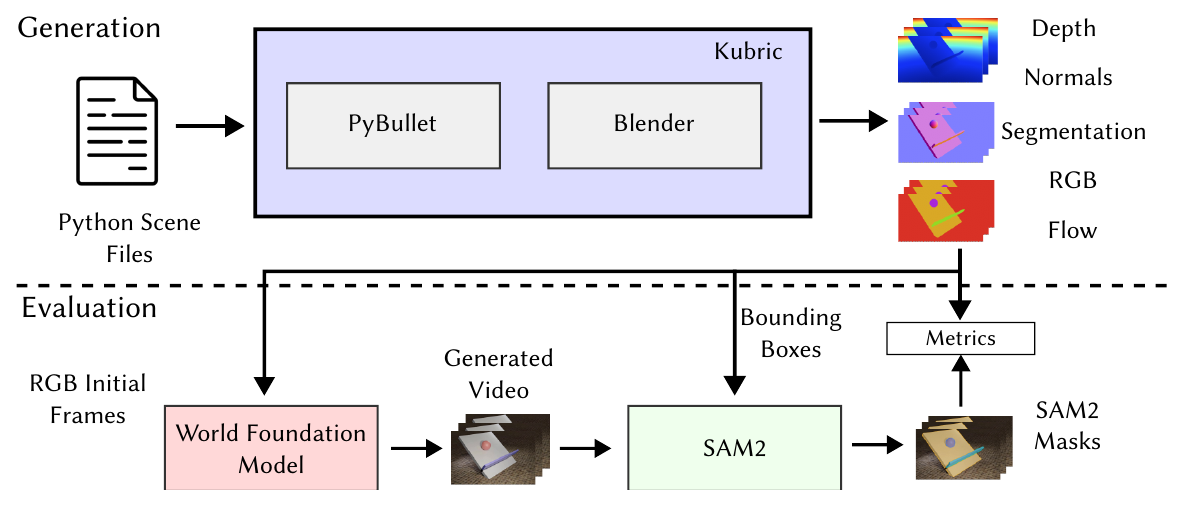
Overview of generation and evaluation. For generation (top), we use Kubric (PyBullet + Blender). During evaluation (bottom), the initial frames are passed to the world foundation model, which completes the video. The completed video is passed to SAM2 along with bounding boxes from ground-truth masks; SAM2 segmentations are compared to ground truth to obtain the final metrics.
Motion physics
Kinematics and dynamics in the generated video, including gravity, friction, and collision. Three scenarios: bouncing ball, two-object fall, and two-object parabolic motion.
Object permanence
Objects continue to exist in the scene even when hidden from the camera. Five scenarios: block & object, columns, raised-block bounce, wall bouncing, and two-ball bounce.
Support relations
How objects physically support one another, including when configurations are stable vs. unstable. Three scenarios: dominoes, ramp block, and table drop.
Perspective / scale
Accuracy of an object’s appearance—size and location—with respect to the camera viewpoint. Two scenarios: object/sphere moving toward the camera, and object/sphere moving away.
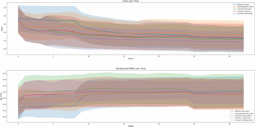
Evaluation compares ground-truth object segmentations with segmentations from the generated videos. Ground-truth masks yield bounding boxes in the first frame; we prompt SAM2 with those boxes and propagate through the rest of the video. Every frame is scored with foreground mIoU. We additionally use the background region (pixels not part of any object mask) to compute background RMSE; because backgrounds remain constant, this measures how well models maintain the background.
Sample videos
Kubric ground truth for each scenario. The figures show typical model rollouts on the same setups; as noted in the paper, results vary greatly between generations.
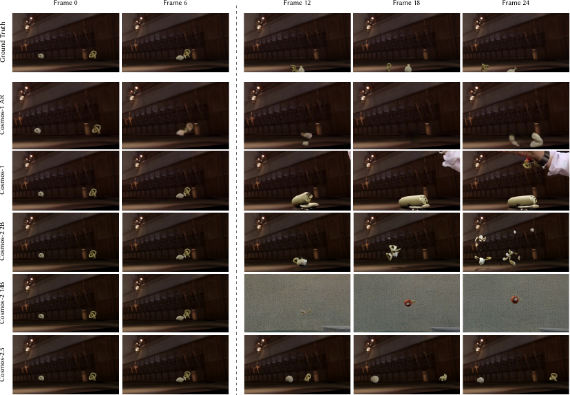
Motion physics. Two objects (a vase and a knot) are thrown at each other, collide, and then fall to the floor. The auto-regressive model greatly distorts the object shapes, while the diffusion model hallucinates the vase into a tank and adds a human hand.
Bouncing ball
A sphere, initially at rest at a known height, falls freely under gravity. Height and restitution are randomized. The prefix includes frames after the first bounce.
Two-object fall
Two objects at different heights and a slight horizontal offset are released to fall under gravity and typically collide with each other and the ground.
Two-object parabola
Two objects on opposite sides are projected toward each other at randomized launch angles and speeds, not necessarily in the same vertical plane.
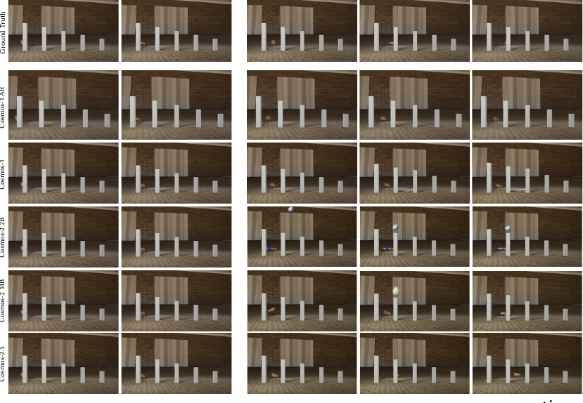
Object permanence. An object is thrown behind a sequence of thin columns, appearing and disappearing as it goes.
Block & object
An object translates left to right behind a wall. It disappears behind the wall and must reemerge on the far side with consistent velocity.
Columns
An object moving left to right behind several thin columns, periodically disappearing and reappearing as it passes each column.
Raised-block bounce
A sphere bouncing vertically behind a raised block. It is periodically occluded at mid-height and not visible to the camera.
Wall bounce
A sphere rolling horizontally behind a block between two walls. It collides with a wall, bounces, and rolls back, reappearing in the gap as it approaches a wall.
Two-ball occlusion
Two spheres bouncing vertically, with a larger sphere in front. The smaller sphere is periodically occluded as their vertical positions diverge.
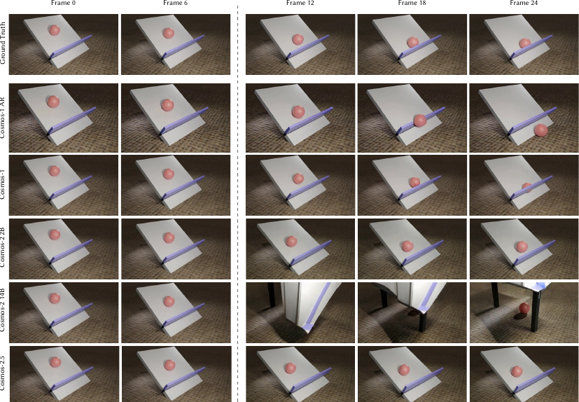
Support relations. A ball is rolled down a ramp toward a solid block near the bottom. Models often handle the roll but miss the interaction with the barrier.
Dominoes
An object collides with a series of standing blocks. Depending on initial velocity, it knocks over a varying number of them, which may subsequently topple onto one another.
Ramp + barrier
A sphere rolls down an incline until a fixed barrier at the end stops it—testing both whether the incline supports the ball and whether the block stops it.
Table drop
An object at a table’s edge with a portion extending beyond the surface. Mere contact is insufficient—the object requires adequate support distribution relative to its mass.
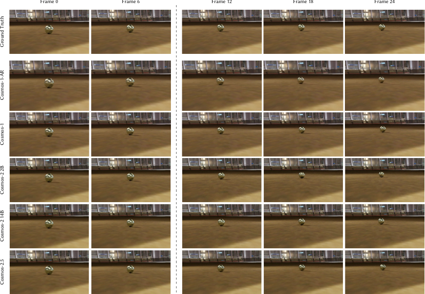
Scale / perspective. A metallic sphere is rolling away from the camera. Apparent size should decrease with distance due to perspective.
Toward camera
A single object is launched from the background and moves toward the camera. As it approaches, it should appear to increase in size due to perspective.
Away from camera
A single object moves away from the camera. As it recedes, it should appear to decrease in size due to perspective.
Auxiliary maps
Synthetic clips also include depth, surface normals, optical flow, and segmentation. One bouncing-ball example:
RGB
Rendered appearance (same clip as bouncing ball above).
Depth
Per-pixel distance from the camera.
Normals
Surface orientation at each pixel.
Optical flow
Forward flow between consecutive frames.
Results
Quantitative results are shown in Table 2 (simulated) and Table 5 (real). Higher is better. Cosmos-1 (33 frames) is strongest overall at 0.45 mIoU. Models perform similarly on the synthetic and real versions of the subset, suggesting that poor performance is not a distribution gap between real video and synthetic test cases but rather poor physics understanding.
Models perform better on scenarios with longer object interaction (Ramp, Table, Walls) than on shorter interactions (Two-object fall, Two-object parabolic motion, Dominoes). They also rely heavily on training priors: a ball rolling down a ramp is handled well, while the uncommon barrier at the bottom of the ramp is not. In a 50-person study, foreground mIoU correlates with human judgments of motion quality (r = 0.846), realism (0.768), overall quality (0.713), and consistency (0.662).
Foreground mIoU on the Physical Principles Understanding subset (simulated videos; Table 2). Since the diffusion models generate 121 frames vs. 33 for the autoregressive model, we provide both comparisons. Category scores on the compact table are unweighted averages of the scenarios in that concept. Higher is better.
Model
Params
Motion
Permanence
Scale
Support
Overall
Cosmos-1 AR
5B
0.290
0.402
0.456
0.545
0.423
Cosmos-1 (33F)
7B
0.318
0.459
0.520
0.478
0.451
Cosmos-1 (121F)
7B
0.170
0.328
0.189
0.320
0.257
Cosmos-2
2B
0.169
0.362
0.347
0.380
0.320
Cosmos-2
14B
0.176
0.255
0.302
0.339
0.268
Cosmos-2.5
2B
0.221
0.376
0.346
0.434
0.349
Per-scenario breakdown (Table 2)
Model
Ball
2-fall
2-para
Block
Cols
Raised
Walls
2-ball
Obj→
Obj←
Sph→
Sph←
Dom.
Ramp
Table
Avg
Cosmos-1 AR 5B
0.376
0.268
0.227
0.264
0.703
0.380
0.500
0.161
0.298
0.412
0.635
0.480
0.461
0.529
0.644
0.423
Cosmos-1 33F 7B
0.372
0.299
0.283
0.348
0.735
0.456
0.558
0.201
0.327
0.484
0.712
0.555
0.489
0.486
0.457
0.451
Cosmos-1 121F 7B
0.164
0.144
0.201
0.205
0.558
0.319
0.416
0.140
0.100
0.233
0.245
0.177
0.157
0.380
0.422
0.257
Cosmos-2 2B
0.190
0.178
0.140
0.127
0.696
0.451
0.330
0.206
0.159
0.434
0.460
0.334
0.243
0.408
0.491
0.320
Cosmos-2 14B
0.191
0.201
0.135
0.167
0.476
0.185
0.270
0.175
0.148
0.371
0.372
0.317
0.207
0.405
0.406
0.268
Cosmos-2.5 2B
0.200
0.304
0.161
0.099
0.736
0.448
0.393
0.206
0.134
0.432
0.500
0.319
0.298
0.505
0.498
0.349
Foreground mIoU on the Physical Principles Understanding subset (real videos; Table 5). Higher is better.
Model
Params
Motion
Permanence
Scale
Support
Avg
Cosmos-1 AR
5B
0.383
0.347
0.163
0.752
0.411
Cosmos-1
7B
0.216
0.364
0.044
0.636
0.315
Cosmos-2
2B
0.293
0.364
0.091
0.765
0.378
Cosmos-2
14B
0.272
0.370
0.084
0.652
0.344
Cosmos-2.5
2B
0.290
0.311
0.091
0.669
0.340
Foreground mIoU and background RMSE over time. Foreground mIoU is inversely related with how far in the future the model is predicting. There is a sharp drop-off after frame 5 or frame 9, when the model first begins predicting (depending on the model). The shaded region is one standard deviation.
PerfectPhysics
The second subset shifts the focus from core physics principles to exact parameter estimation. One key goal of world foundation models is replacing physics simulation software (where parameters are hard-coded or manually tuned) as a synthetic data generator. To that end, it is crucial that these models generate videos with accurate values for key physical parameters, such as gravitational acceleration.
We designed three experimental setups testing gravitational acceleration, friction coefficients, and fluid viscosity: 51, 103, and 80 videos respectively, for a total of 234 real videos. We additionally generate 30 gravity and 15 friction videos synthetically, bringing the combined total to 279. We validate the estimation pipeline by running it on our collected videos and ensuring that the output is close to ground truth (e.g. 9.81 m/s2 for gravitational acceleration); see Table 1 of the paper.
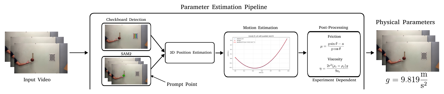
Overview of the physical parameter estimation pipeline. Given an input video, we first use checkerboard detection and SAM2 to extract 3D positions for objects. We then fit curves to these trajectories to estimate relevant physical properties such as acceleration or terminal velocity, and post-process them, if needed, to calculate the reported physical parameters.
Gravity · 51 real + 30 sim
17 straight drops and 34 parabolic launches. For free-fall, an object is dropped from rest; the video is trimmed so the initial frame is already freely in the air. For parabolic motion, objects are pushed up a ramp and fall toward the ground, again trimmed to free flight. Target: 9.81 m/s2.
Friction · 103 real + 15 sim
A steel cube slides down a ramp covered with wood (30), rubber (19), sandpaper 80 grit (18), sandpaper 3000 grit (18), or plastic (18). The ramp angle varies between runs. We recover the kinetic friction coefficient from the acceleration: μ = (g sinθ − a) / (g cosθ).
Viscosity · 80 real
A steel ball is dropped into a beaker of glycerine (32), corn syrup (30), or honey (18). The video is trimmed so the object is already at terminal velocity in the first frame. Viscosity follows from Stokes’ law: η = 2r2(ρs − ρf)g / 9vt. Videos were collected at 75°F in a single session.
Extracting constants from monocular video requires camera intrinsics/extrinsics, the 2D pixel location of the object, and depth. Intrinsics come from a traditional checkerboard calibration; a checkerboard in every scene yields extrinsics. SAM2, prompted by a manually selected point, tracks the object; we take the centroid of the mask as its 2D location. Depth is held constant by moving objects in a plane parallel to the camera. Gravity and friction use a quadratic fit to positions over time; viscosity uses a linear fit for terminal velocity.
Sample videos
Real lab footage next to Cosmos-2.5 and Wan 2.2 continuations of the same setups. Video-to-video models receive enough input frames to estimate the correct constant; image-to-video models see only the first frame.
Ground-truth free-fall
Object dropped from rest; the prefix starts already in free flight. Pipeline recovers 9.78 ± 0.38 m/s2 on real footage (GT 9.81).
Cosmos-2.5
Models tend to exhibit realistic motion paths (straight drops, parabolas) while failing to abide by 9.81 m/s2.
Wan 2.2
Image-to-video from the cropped first frame. Lack of temporal information leads to severely low or even negative gravity estimates.
Parabolic motion
Objects are pushed up a ramp and fall toward the ground. 34 real clips; the prefix starts already in free flight. Ramp angle is randomized.
Cosmos-2.5 parabola
Same launch, world-model continuation. Realistic trajectory is not the same as the correct g.
Cosmos-2 parabola
Same launch, Cosmos-2 2B continuation. Realistic trajectory is not the same as the correct g.
Ground-truth wood
A steel cube sliding down a wood ramp. Real-video estimate μ = 0.35 ± 0.05 (accepted range 0.2–0.5). Ramp angle is randomized.
Cosmos-2.5
Same ramp. Models typically produce a sliding object but not the correct μ; long-tail surfaces such as plastic collapse toward the mean.
Wan 2.2
Image-to-video from the first frame of the same clip. Distant friction pairs (e.g. rubber vs. plastic) are ranked more reliably than close ones.
Ground-truth honey
Steel ball at terminal velocity in honey. Real-video estimate η = 13.82 ± 0.75 Pa·s (GT 14.1)—far from average fluids.
Cosmos-2.5
Continuation of the same drop. Models typically cannot simulate long-tail materials such as honey and instead pull them toward the average.
Wan 2.2
Image-to-video from the first frame. Across models, viscosity rankings among glycerine, corn syrup, and honey are near chance.
Results
Across the board, models both estimate parameters poorly and exhibit extremely high variance. Experiments in this subset are highly constrained in an effort to focus solely on the parameter being tested. Despite this, all models—Cosmos-family and image-to-video—show extremely high variance between rollouts. This is especially apparent in gravity, where objects experience downward acceleration at varying levels even between rollouts with the same object and trajectory.
Model outputs tend to follow realistic motion trajectories while not adhering to realistic motion parameters. For gravity, all models tended to exhibit realistic motion paths most of the time (parabolic trajectories and straight drops). However, they fail to abide by 9.81 m/s2. Similar trends appear for viscosity and friction. Visual realism alone is not sufficient for synthetic world-data generators.
Estimated g on real free-fall
Ground truth
9.81
Our real videos
9.78 ± 0.38
Cosmos-2 2B
8.93 ± 4.79
Cosmos-2 14B
8.43 ± 3.48
Cosmos-2.5
4.78 ± 4.47
Kling 3.0
4.46 ± 1.32
Cosmos-1 AR
4.22 ± 3.71
Runway 4.5
1.48 ± 2.71
Wan 2.2
0.38 ± 0.78
CogVideoX
−0.04 ± 0.14
059.8114
m/s2
Whiskers are one standard deviation. Scale is 0–14 m/s2 so the ±4.79 spread on Cosmos-2 2B is visible; whiskers that would go below 0 are clipped. Image-to-video models suffer from lack of temporal information in the input; this is exacerbated on gravitational acceleration, where estimates are severely low or even negative.
Estimated physics parameters on the physical parameter estimation subset (real videos; Table 3). Ground-truth ranges and our real-video estimations are provided as comparison. For gravity and viscosity, models closest to ground truth are bolded. Due to the wide range of acceptable friction values, models closest to our real-video estimations are bolded. Units: m/s2, Pa·s, dimensionless μ. SP stands for sandpaper.
Model
g fall
g para
η glyc
η syrup
η honey
μ wood
μ rubber
μ SP80
μ SP3k
μ plastic
Ground truth
9.81
9.81
1.2
6.0
14.1
0.2–0.5
0.5–2.0
0.7–1.1
0.2–0.5
0.05–0.2
Real videos (ours)
9.78±0.38
9.85±0.36
1.22±0.01
5.84±0.02
13.82±0.75
0.35±0.05
0.93±0.10
1.06±0.05
0.30±0.02
0.22±0.03
Cosmos-1 AR
4.22±3.71
4.30±1.29
7.80±1.04
8.44±2.11
>50
0.54±0.12
1.24±0.14
1.28±0.19
0.53±0.08
0.51±0.10
Cosmos-1 DM
3.51±1.91
7.65±2.93
0.60±1.19
1.54±1.48
0.17±0.17
0.67±0.17
1.30±0.21
1.45±0.26
0.52±0.14
0.48±0.12
Cosmos-2 2B
8.93±4.79
8.23±3.81
0.25±0.39
1.09±0.31
9.85±6.20
0.70±0.09
1.47±0.26
1.26±0.26
0.60±0.11
0.61±0.13
Cosmos-2 14B
8.43±3.48
9.15±4.17
0.22±0.10
1.30±0.84
1.81±1.81
0.66±0.16
1.22±0.41
1.14±0.47
0.56±0.09
0.46±0.39
Cosmos-2.5
4.78±4.47
5.38±2.76
0.80±0.48
1.09±0.31
1.68±0.08
0.70±0.19
1.45±0.34
1.52±0.28
0.61±0.12
0.63±0.14
Wan 2.2
0.38±0.78
1.68±3.07
3.42±5.12
3.16±3.17
3.28±2.76
0.67±0.10
1.32±0.22
1.48±0.24
0.52±0.16
0.58±0.11
Hunyuan
0.37±0.79
0.21±0.41
7.20±3.71
>50
>50
0.66±0.09
1.43±0.23
1.05±0.22
0.53±0.08
0.57±0.10
CogVideoX
−0.04±0.14
0.18±0.24
3.29±2.85
2.25±2.77
2.67±1.91
0.63±0.13
1.47±0.33
1.29±0.50
0.52±0.13
0.50±0.20
Runway 4.5
1.48±2.71
3.55±1.12
1.96±0.77
3.37±1.12
2.87±0.69
0.91±0.40
2.32±0.93
0.30±0.52
0.79±0.25
0.61±0.28
Kling 3.0
4.46±1.32
2.92±0.77
2.57±0.87
1.95±1.57
1.34±0.99
0.75±0.97
1.88±0.67
1.26±1.04
1.78±0.82
0.44±1.44
LTX-2.0
0.48±0.97
3.77±0.74
0.97±0.35
3.45±1.42
3.37±2.78
0.42±1.67
0.34±3.79
0.22±0.57
0.27±0.70
1.48±1.67
Estimated physics parameters on the physical parameter estimation subset (simulated videos; Table 4). Various materials are tested for friction; we report average RMSE. Values closest to ground truth or with the lowest error are bolded.
Model
Params
Free-fall (m/s2)
Parabolic (m/s2)
Friction error ↓
Ground truth
9.81
9.81
—
Cosmos-1 AR
5B
10.83±2.93
7.41±1.15
0.298
Cosmos-1 DM
7B
7.53±3.67
6.27±1.60
0.231
Cosmos-2
2B
4.29±5.06
13.23±4.31
0.232
Cosmos-2
14B
4.23±6.74
2.93±3.02
0.274
Cosmos-2.5
2B
10.49±3.93
12.54±3.30
0.217
Wan 2.2
5B
1.16±2.63
0.06±1.03
0.253
Hunyuan Video
13B
0.94±0.72
0.68±0.57
0.228
CogVideoX
5B
−0.23±2.39
0.31±1.63
0.361
Runway Gen-4.5
—
1.23±1.17
3.12±2.55
0.317
Kling 3.0
—
5.84±2.55
4.60±3.67
0.436
LTX-2.0
14B
0.57±0.35
2.79±2.43
0.243
Conclusion & Takeaways
WorldBench aims to provide a benchmark to separate visually convincing video from physically correct video. Instead of a single entangled score, each clip tests one concept or constant, and relies on objective metrics from the simulator or real physical constants. By evaluating SoTA video to video and image to video models, we find the following conclusions:
Rollouts often look right (a ball follows a parabola) while the numbers are wrong (it does not fall at 9.81 m/s2).
Recovered parameters are biased and extremely high-variance, even across rollouts of the same scene.
Image-to-video models are especially weak on gravity: with only a first frame, estimated g is often far too small, or even negative.
Long-tail materials collapse toward the mean. Honey (very viscous) and plastic (very low friction) are simulated like more ordinary fluids and surfaces, without extra variance.
Scores are similar on synthetic and real tests, so the gap is physical understanding, not a renderer mismatch.
Data
worldbenchmark/WorldBench
— intuitive physics (motion, permanence, support, scale), with masks and auxiliary maps. 132-frame sequences; ShapeNet objects. Prompts used in the paper will ship with the public codebase.
worldbenchmark/PerfectPhysics
— gravity, friction, and viscosity lab videos used to estimate g, μ, and η. Evaluation code for recovering constants from video will ship with the public codebase.
BibTeX
@article{upadhyay2026worldbench,
title={WorldBench: Benchmarking Physical Understanding of World Models by Isolating Physics Concepts},
author={Upadhyay, Rishi and Zhang, Howard and Solomon, Jim and Agrawal, Ayush and Ba, Yunhao and Wong, Alex and de Melo, Celso M and Kadambi, Achuta},
journal={arXiv preprint arXiv:2601.21282},
year={2026}
}